The ionozond Playground: An HF Channel Simulator — a Real Sounding and Twelve Copies of It

An HF modem or algorithm is tested on a simulator, not on the air: the air never repeats, and two variants cannot be compared on the same path in the same hour. The classic models — Watterson’s and those of ITU-R F.1487 — define the channel by a table: two paths of equal power, a fixed delay difference and a Doppler spread for “quiet”, “moderate” and “disturbed” conditions. Such a channel is convenient for comparing modems, but it does not look like any particular path at any particular hour.

The muf.sim simulator works the other way round: it takes the channel’s parameters from an oblique chirp sounding of the same path. The simulator itself is not published yet. The playground gained two pages about it: “Channel simulator” shows its results on real soundings, and “Simulator: notes” explains how it works.

Does the real sounding pass for a copy

The key device is a self-check. A synthetic sounding is written in the same .lfs format as a real recording and goes through the same processing: the same trace extractors, the same tracker, the same interference cleaning. So a copy compares with the original directly, bin for bin. If the channel state is complete, the real sounding should pass for one more copy. How far it is from that is what the page shows.

The chain goes like this. A channel state is built from the real sounding: a list of modes, and each mode is not a set of numbers but a set of curves over frequency — delay, carrier-to-noise density C/N₀, Doppler, delay spread. Every quantity carries a provenance tag: measured off the sounding, a prior, or set by a model. Twelve copies of the sounding are synthesised from the state, differing only in fading and noise. Each copy is read back through the same processing — that is level 1, recovery. Then the real sounding is put among the copies — level 2, realism.

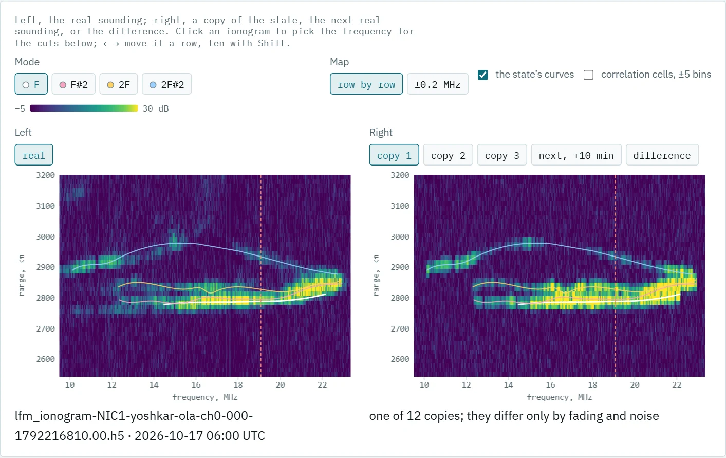
Two ionograms of range from 2550 to 3200 km over frequency from 10 to 23 MHz: left, the real sounding, right, a copy; both show two bright traces near 2780 and 2830 km and a weak trace rising to 2980 km near 15 MHz, with smooth coloured mode curves over the traces; above, switches for the modes F, F#2, 2F, 2F#2, the “row by row” and “±0.2 MHz” maps, and for the right panel: copies 1–3, the next sounding 10 minutes later, and the difference — 17 October, 06:00 UTC. Left, the real sounding; right, copy 1; the coloured lines are the state's mode curves, the orange dashes the chosen frequency.

The copy reproduces both traces and their level, but draws them smooth: the original’s patches and kinks are not in the state. The right panel can also show the next real sounding, 10 minutes later — two versions of “the same channel” — or the difference “real minus copy”. Below come a range cut at the chosen frequency, C/N₀ along a mode, the profile across the trace, the ionogram correlation, the state table, and

H(f, t)

— what a signal 48 kHz wide would see at one carrier over 30 seconds.

A power ionogram cannot measure the Doppler shift, the fading law or the split into ordinary and extraordinary waves. In the state these quantities are priors, by default F.1487’s “moderate mid-latitude conditions”: a 0.5 Hz spread, a Gaussian spectrum, Rayleigh fading. The state table marks them so.

A verdict in sigmas

Level 2 compares the MUF, the level scatter along the trace, the trace width and the ionogram correlation — row by row and after averaging over ±0.2 MHz. Every verdict follows one rule: the real value’s distance from the copies’ mean is measured in the standard deviations one more copy would have, with a factor √(1 + 1/n) for the error of the mean itself. “Inside” means

≤ 3. For a correlation the rule works on Fisher’s z-transform and is one-sided: a real sounding more like the copies than they are like each other is no defect.

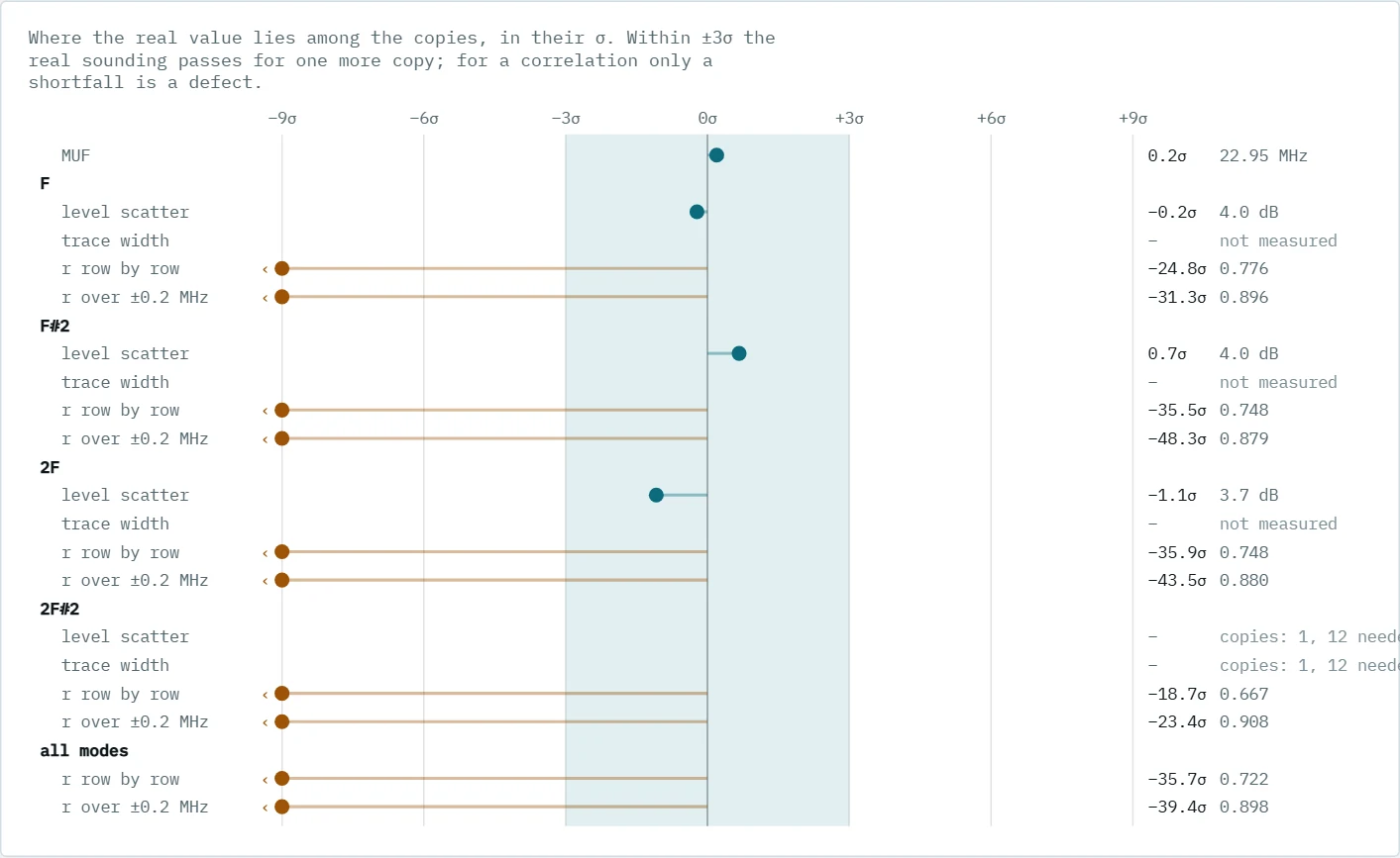
A z axis from −9σ to +9σ with a shaded ±3σ band: the MUF at +0.2σ and the level scatter of three modes from −1.1σ to +0.7σ as teal dots inside the band; correlations row by row and over ±0.2 MHz for the modes F, F#2, 2F, 2F#2 and all modes as orange dots with arrows beyond −9σ, from −18.7σ to −48.3σ; on the right, the z values and the quantities — Level-2 verdicts for the 06:00 sounding: the MUF and level scatter inside the ±3σ band, the correlations far to the left.

The threshold is 3σ rather than 2σ because the tails are heavy: at 2σ true copies were called “outside” 13 times in 160, at 3σ 5 times. The rule is calibrated on true copies: one more sounding was synthesised from the state and read as if it were real, 25 times for each of three February states. The earlier rule, “inside the copies’ [min, max]”, called a true copy foreign 2/(n + 1) of the time — with three copies, every other time.

A large

for a correlation says the difference is easy to see, not that it is large. Twelve copies over ten thousand cells agree with each other to ±0.005, so a gap of 0.1 makes tens of sigmas. The gap’s size is read off the correlation bars.

What the soundings of 17 October showed

The built-in data are four soundings of the NIC1 — Yoshkar-Ola path: 06:00, 09:00, 12:00 and 18:00 UTC, with 12 copies each.

The MUF is reproduced. In all four soundings the real MUF lies inside the copies’ scatter, z from +0.2 to +1.3. The MUF itself moves by 0.4–1.4 MHz in 10 minutes.
A copy is no worse than the next sounding. Row by row, the copies correlate with the original almost as well as the real sounding 10 minutes later: 0.72, 0.70, 0.71 and 0.63 against 0.71, 0.71, 0.69 and 0.58. The state describes its moment no worse than the channel keeps itself over one repeat.
But the copies are more alike. The gap to the “ceiling” — the copies’ mean correlation among themselves — is 0.07–0.13. The real ionogram holds structure the state lacks: the trace is 15–32 µs wider than a point echo and wanders smoothly around a smooth curve from row to row. That is why almost only the correlations end up outside.
Split modes give +3 dB. Where the tracker split one trace into two modes over nearly one band at nearly one delay, the state holds two equal paths instead of one, and the copy’s C/N₀ comes out 3.1–4.4 dB high. Modes that overlap nothing come back to about 1 dB.
The delay is recovered with an rms of 9–30 µs — within a range bin of 48.8 µs. At the MUF, where the rays meet, the error reaches hundreds of microseconds: the tracker hands parts of one branch to the other, on the copies just as on real soundings. The tracker’s error can only be measured on a sounding whose answer is known, which is a side benefit of the simulator.

The notes and six boards

The “Simulator: notes” page takes everything in order: the model, synthesis, checks, a guide to the page, the October results and the limits. The basics rest on six boards. All of them are computed, not drawn: a simulated beat signal of a four-mode channel is run through the station’s processing — 100 kHz/s, 40 kHz after decimation, a Hann window of 16,384 samples.

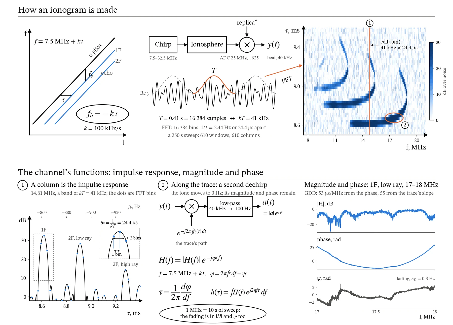
A board in two rows. Top: the chirp replica and an echo as parallel lines in the time–frequency plane, fb = −kτ; the chain “chirp — ionosphere — multiplication by the replica — y(t)”; a window of the beat signal and a model ionogram with a column and a stretch of trace marked. Bottom: an ionogram column as the impulse response, with FFT bins as dots and a loupe on one 24.4 µs bin; the second dechirp along the trace; magnitude, phase and the phase remainder over 17–18 MHz — Board 1: how an ionogram is made and what is read from it — the impulse response, and a mode's magnitude and phase.

The first board goes from the chirp to the ionogram, and from the ionogram to the channel’s functions: an ionogram column is the channel’s impulse response within 41 kHz. It also explains how an FFT bin differs from the resolution. Neighbouring bins are 1/(kT) = 24.4 µs apart, but the Hann window widens a peak to about two bins, and two equal paths show a dip between their peaks only when about 2.5 bins, or 60 µs, apart. An echo between bins loses up to 1.4 dB, and the maximum of the noise over many bins sits further above the median the more bins there are — so a detection threshold depends on how many bins are searched. The earlier claim that paths 24.4 µs apart already separate is corrected.

The second board takes apart, step by step, the second dechirp that reads a mode’s magnitude and phase off a sounding. After the first dechirp a mode is a tone, but the tone drifts along the trace: over 17–18 MHz, from −865 to −870 Hz in 10 seconds. Multiplying by the conjugate path brings the tone to zero, a low-pass filter keeps ±50 Hz around zero — the complex envelope a(t) — and the dispersion from the phase’s curvature, 53 µs/MHz, agrees with the trace’s slope, 55 µs/MHz. There is a caveat: on an up-sweep frequency and time are tied together — 1 MHz takes 10 seconds — so one sounding cannot tell frequency selectivity from change over time.

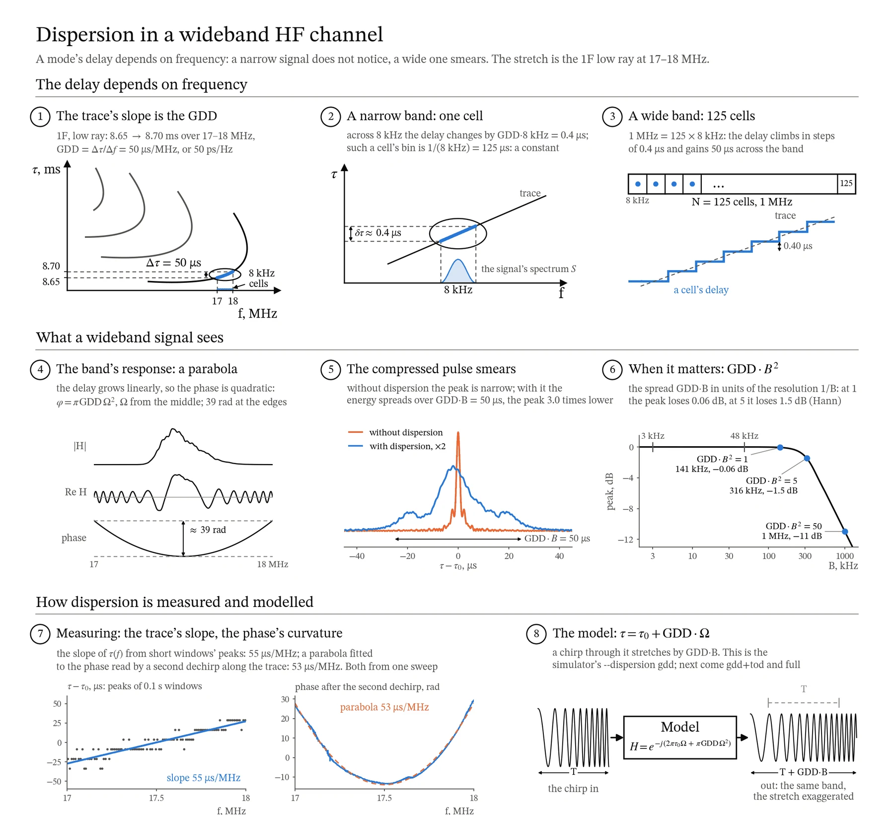
The board “Dispersion in a wideband HF channel” in eight numbered steps across three rows: the trace's slope as the GDD, a narrow band within one cell and a wide band of 125 cells; the phase parabola, the smearing of a compressed pulse and the peak loss against GDD·B²; measuring by the trace's slope and by the phase's curvature, and the model in which a chirp stretches by GDD·B — Board 3: what 50 µs/MHz of dispersion does to a signal — eight steps in three rows.

The third board is about dispersion within a mode. Across an 8 kHz cell the delay changes by only 0.4 µs, and to such a signal the channel is just a delay. But 1 MHz is 125 cells, and over them the delay climbs a staircase by the full 50 µs. How much this matters is told by GDD·B²: at 1 the peak loses 0.06 dB, at 5 it loses 1.5 dB. On this stretch those are bands of about 140 and 320 kHz, while signals 3 and 48 kHz wide do not notice the dispersion. The last step shows how a chirp stretches in such a model — the stretch is drawn exaggerated: on a 10-second sweep it is 50 µs.

Boards 4 and 5 are about the slow and fast parts of the state. The slow part — traces, level and width — comes from the power ionogram: C/N₀ is collected over five bins around the trace, because the Hann window smears an echo over a bin and a half. The fast part — the Doppler spread, the spectrum’s shape, the Rice factor and the o/x split — can only be measured from the recording’s phase. Two waves 30 µs apart beat along the sweep at kΔτ = 3 Hz, and read as one wave they give a spread many times too wide: on the board, 3.0 Hz instead of 0.3. So the estimate fits a pair of waves too.

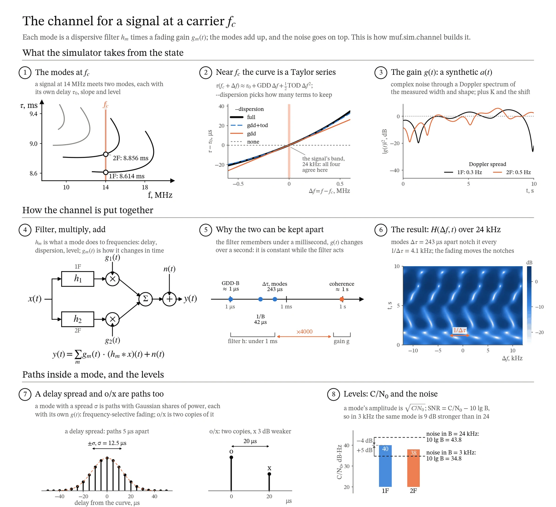
The board “The channel for a signal at a carrier fc” in eight steps: the modes at 14 MHz with delays of 8.614 and 8.856 ms; the curve's Taylor expansion and four dispersion settings; the fading gain g(t) of two modes; a block diagram “filter — multiply — add — noise”; a time scale from 1 µs to 1 s with a factor of 4000 between the filter's memory and the coherence time; a map of |H| over frequency and time with notches every 4.1 kHz; a delay spread and an o/x pair as sets of paths; C/N₀ levels and the noise in 3 and 24 kHz bands — Board 6: the channel for a signal at one carrier — a mode's filter, a fading multiplier and the sum of the modes.

The sixth board shows how the simulator builds a channel for a modem. Each mode is a dispersive filter fixed in time, multiplied by a fading gain; the modes add up, and the noise goes on top. Splitting into a filter and a gain is exact as long as the gain does not change while the filter responds: the filter remembers under a millisecond, while the fading’s coherence time is about a second, 4000 times longer. Two modes 243 µs apart cancel each other every 4.1 kHz, and the fading moves these notches across the band. A signal 3 kHz wide fades as a whole, while a 24 kHz band holds about six notches at once — the modem needs an equaliser.

What the simulator cannot do yet

The notes list the limits plainly. One up-sweep cannot tell a Doppler shift from a change of delay, so the shift stays a prior. The trace’s fine structure — its wander around a smooth curve — is not modelled, and it is exactly what makes the gap to the ceiling. The noise is synthesised white, without broadcast stations or impulsive interference. A state describes one moment; the next stage is series of states and a forecast of the next one.

Work on the boards also corrected the text itself. Dispersion within one FFT window is now computed as GDD·kT — 0.6 µs, not GDD·(kT)²; the mention of “hundreds of microseconds” of dispersion is gone; the noise term was added to the received signal’s formula. And the first version of the synthesis faded a mode inside its band and set every copy’s MUF 0.03 MHz low — the level-2 check found it.

Conclusions

A simulator built from a sounding of the same path checks itself: if the state is complete, the real sounding should pass for one more copy.
The yardstick is the next real sounding: a copy as close to the original as the channel is to itself 10 minutes later describes the moment well enough.
A verdict in the sigmas of one more copy, calibrated on true copies, is fairer than “inside the copies’ range”.
Boards computed through the same processing as the data also check the text that explains them: work on them found errors in the notes’ formulas.

Availability

The page draws what the simulator computed and computes nothing itself. The built-in data are ionograms of real soundings; your own data can be loaded on the page from a JSON file, and they stay in the browser.

Playground: konkin-nikita.ru/ionozond-playground — the “Channel simulator” and “Simulator: notes” pages
Playground source code: github.com/nikita-konkin/ionozond-playground
Console and document: github.com/nikita-konkin/ionozond