The ionozond Playground: Dispersion, Ionogram Cells and a Day on the Path, in Models You Can Move

The ionozond console comes with a document, “Oblique Chirp Ionograms”: how a chirp ionogram forms, what its traces mean and where the picture can mislead. The document is detailed but static: a formula shows a relationship, not how it behaves at another frequency or another bandwidth. The playground is seven models for its parts, where the parameters move on sliders and the charts recompute at once.

The playground is a static site in Russian and English. No build, no server, no external libraries: plain scripts, with the charts drawn by hand in SVG. It opens with a double click on index.html or online — the site is published from the main branch through GitHub Actions, and the footer gives the published commit and its date.

Dispersion on the ionogram

The main model is about group-delay dispersion (GDD) — the slope of a trace on the ionogram, dτ/df. It decides how wide a band the path carries undistorted: across the signal’s band the delay changes, and the pulse comes out smeared.

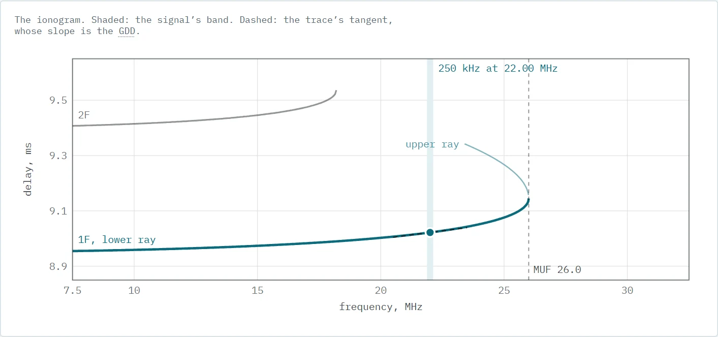
A plot of delay 8.9–9.6 ms against frequency 7.5–32.5 MHz: the 2F trace near 9.4–9.5 ms up to 18 MHz, the lower ray of 1F from 8.95 ms rising towards the 26 MHz MUF where it meets the upper ray; a vertical band for the signal at 22 MHz with a dot and a tangent — A model ionogram of the Cyprus — Yoshkar-Ola path: a 250 kHz signal at 22 MHz with the maximum usable frequency (MUF) at 26 MHz. The dashed line is the trace's tangent; its slope is the GDD.

The model rests on measurements from this path. The law GDD = 7.5·(1/√(1 − f/MUF) − 1) µs/MHz is the median of 19,033 slope estimates from 583 soundings on 4–9 February 2026. The coefficient b was fitted to the medians of 19 f/MUF bins from 0.5 to 0.975, weighted by the number of estimates: b = 7.52 with R² = 0.975; without the weights, or starting the fit at 0.6–0.8 MUF, it comes out at 7.4–7.6. The page says plainly that this is a parameter of one path’s model, not a universal constant, and that the interquartile spread is about ±50 %.

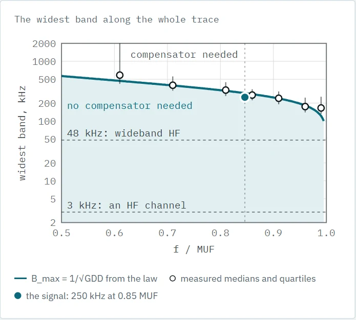
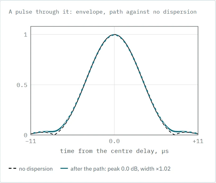
A log-scale plot of the widest band from 2 kHz to 2 MHz against f/MUF from 0.5 to 1: the law falls from 600 to 100 kHz, circles are measured medians with their spread, and the signal's dot at 250 kHz and 0.85 MUF sits in the region where no corrector is needed; dashed lines at 48 kHz and 3 kHz — The widest band along the whole trace: the law and the measured medians with quartiles.

A pulse envelope from −11 to +11 µs: the curve after the path almost coincides with the dashed curve without dispersion; the legend gives a 0.0 dB peak and ×1.02 width — A pulse after the path: at this bandwidth it barely changes.

GDD gives an estimate of the widest band, B_max ≈ 1/√GDD. The playground treats it as a cautious limit, not a cliff: a Python check shows that at GDD·B² = 1 a pulse loses only 0.06 dB, and it degrades noticeably only near 5 — losing 1.5 dB and growing 1.6 times wider. For wideband HF communication with a 48 kHz band, no corrector is needed on this path almost up to the MUF itself.

On the same page a compensator in the receiver can be switched on — an all-pass filter with group delay −GDD_est·(f − f_c), where the GDD estimate carries an error set by a slider. At a 26 MHz MUF and a signal at 0.85 MUF the widest band grows from 293 kHz to 1.45 MHz with an exact estimate, to 710 kHz with a +2 µs/MHz error, the kind left after averaging several soundings, and to 448 kHz with a +5 error, as from a single sounding. Under the cards the calculation unfolds step by step with the page’s current numbers, and where a line subtracts two printed values the result is their difference, so the arithmetic can be checked. The latest change: the signal’s centre can be pinned at 0.85 MUF, and it then follows the MUF as it moves.

Measuring, timing and the schedule

Three pages take apart where the numbers on an ionogram come from.

Measuring GDD. The delay’s slope or the phase’s curvature in a 1 MHz window, over 300 realisations. On this path the phase method loses: with fading at 0.37 Hz the phase wanders during the 10 seconds a 1 MHz window takes, and the parabola reads that wander as dispersion. From one sounding the delay method’s error is about ±4 µs/MHz, the phase method’s ±6–7. The model was checked against full processing of synthetic captures in all four variants, to within 15 %.
chirptime errors. Where the echo goes when the start time or the sweep rate is wrong: 1 ms of offset is 300 km of group path, 0.2 s is the edge of the unambiguous interval, and an error of an even number of seconds lands in the decimator’s null.
The station schedule. The ionozond planner step by step: the nearest start no sooner than 3 seconds ahead, stations skipped while the receiver is busy, and the conversion of rep:offset into chirptime.

FFT length and the cell

An ionogram cell is k·N/f_IF in frequency by f_IF/(k·N) in delay, where k is the sweep rate and N the FFT length. Their product is always one, so the FFT length chooses not precision but a balance between frequency and delay. A new section opens one column at the “nose” of the 1F trace — where the lower and upper rays meet.

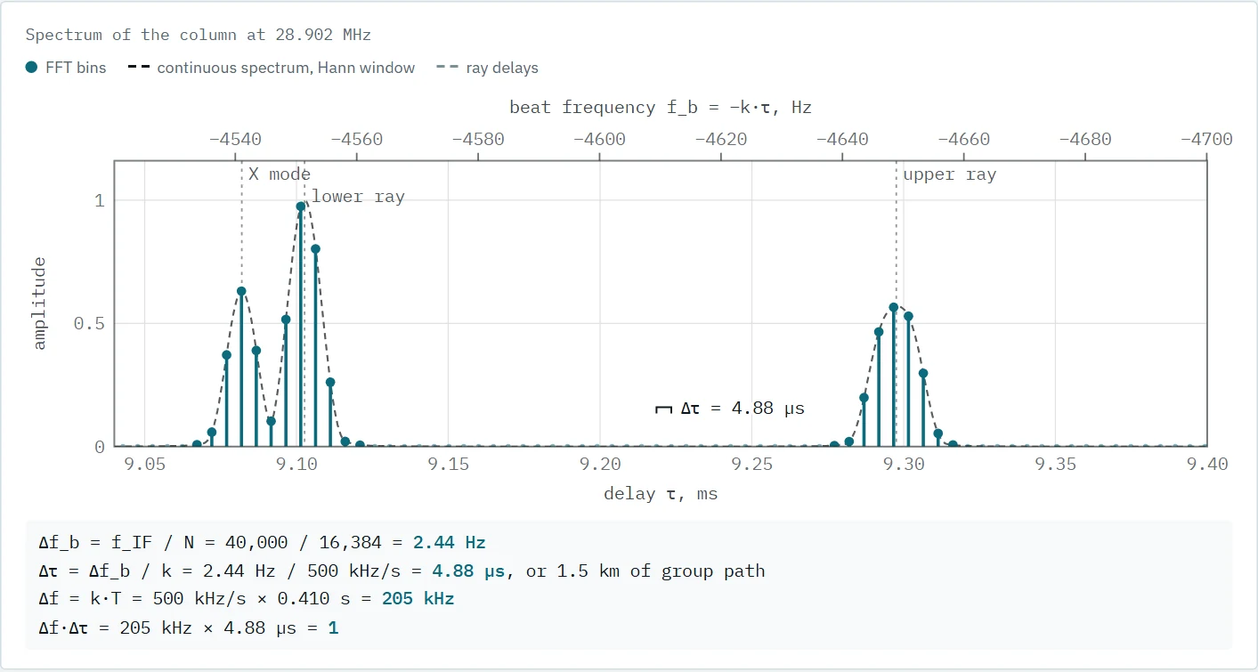
The spectrum of the column at 28.902 MHz over delay 9.05–9.40 ms and beat frequency −4540…−4700 Hz: three peaks — the X mode near 9.08 ms, the lower ray near 9.10 ms and the upper ray near 9.30 ms; a delay step of 4.88 µs; below the plot, Δf_b = 2.44 Hz, Δτ = 4.88 µs, Δf = 205 kHz and Δf·Δτ = 1 — The spectrum of one column at the trace's nose: FFT bins, the continuous spectrum with a Hann window, and the rays' delays. Below, the working of the cell.

The check_cells.py check repeats the section with full processing: a synthetic capture, the FFT, and the console’s own small-object removal. The result is the same as on the page: at 500 kHz/s a 16,384-point FFT erases the trace, while 4,096 points keep it.

A day on the path and vertical sounding

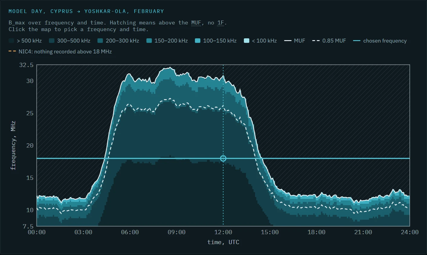
A map of B_max over frequency 7.5–32.5 MHz and time 00:00–24:00 UTC: by day the region under the MUF rises to 30–32 MHz, at night it falls towards 12 MHz; colour shows the band from over 500 to under 100 kHz, narrow right at the MUF; lines for the MUF and 0.85 MUF, a chosen frequency of 18 MHz and the moment 12:00 — A model day on the path in the dark theme: the widest band over frequency and time. Hatching marks frequencies above the MUF, where there is no 1F mode.

The “Day” page shows the MUF’s daily course and a map of the widest band over frequency and time — for the oblique path and for vertical sounding. The model day is a schematic, and the page says so; a real day from the archive can be loaded instead, as JSON prepared by tools/export_daily.py.

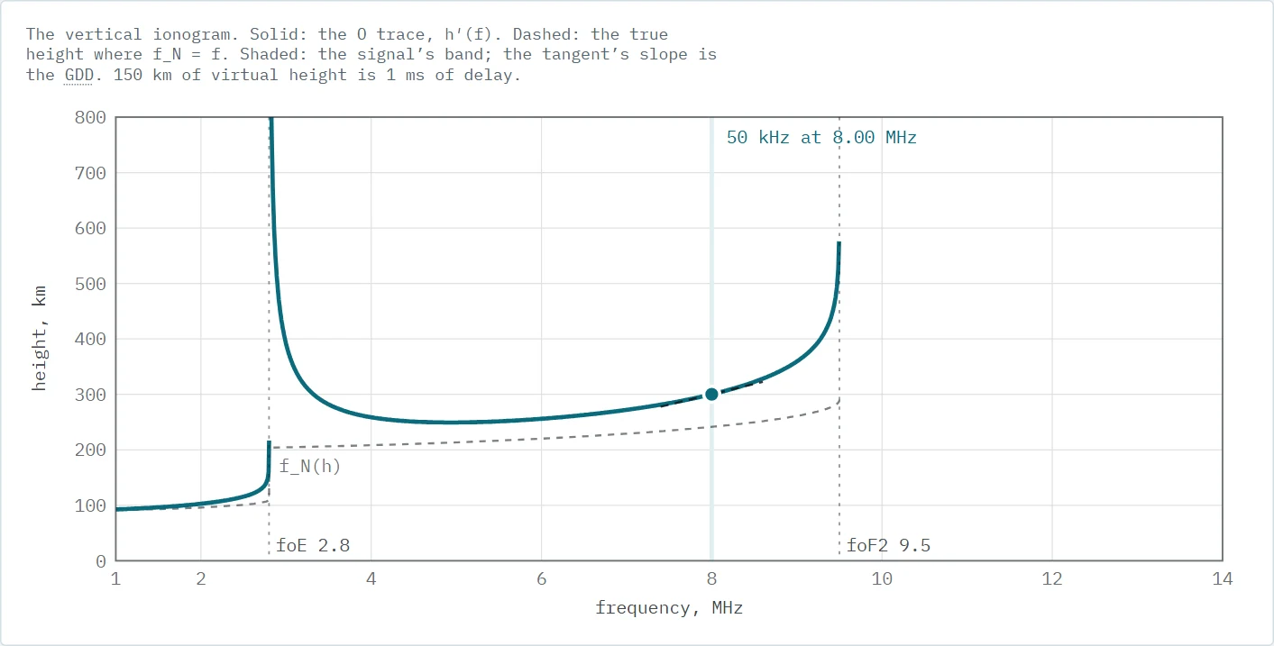
A vertical-sounding ionogram: virtual height from 90 to 800 km over frequency 1–14 MHz; the E trace up to its 2.8 MHz critical frequency, then the F2 trace with a minimum near 250 km rising steeply at the 9.5 MHz critical frequency; a dashed line for the true height; a 50 kHz signal band at 8 MHz — Vertical sounding: an h′(f) ionogram from a model profile of the E and F2 layers. Towards the critical frequencies the virtual height rises, and with it the GDD.

The vertical ionosonde in the model repeats the station in the ionozond schedule: 50 kHz/s, 1–14 MHz. The same ionosphere is carried over to the oblique path by the secant law, and the resulting GDD is compared with the measured law. The Python check agrees with the analytic formula for a single layer to within 0.02 km, and a daytime F2 layer with a weak E layer reproduces the medians from 0.6 to 0.96 MUF to within 2–3 µs/MHz.

The wiki and the glossary

The document’s full text is in the playground as a wiki, in English and in Russian translation. The build script cuts the document into text blocks by their positions in the source, so markup and figures carry over unchanged, and the Russian version substitutes each block’s translation. There are 623 blocks now, none untranslated. Under each part are links to the models that illustrate it.

The glossary covers 16 terms: GDD, MUF and LUF, the trace, the 1F/2F/3F modes, O and X, foF2, chirp, FFT, IF, LO, SNR, chirptime, rep:offset, GPSDO and NTP. In the text of every page the first mention of a term is underlined with dots; hovering or tapping opens a short note with links to the document’s part and the glossary.

The wiki turned out to have an unexpected role — checking the document itself. Work on the models found places that the document’s own tables and formulas contradict. At first the playground corrected them at build time without touching the source: the spacing between modes, the choice of FFT length, the GDD error from one sounding. Then the corrections moved into the document. The build stopped on them — the text to correct was no longer there — and the playground’s patches were removed.

Checking the models

Each model is checked independently by Python scripts in tools/validate/. The checks also show the limits. From 0.61 to 0.96 MUF the GDD law lies inside the measurements’ interquartile range, but at 0.99 MUF it is twice as steep as the median, so near the MUF the pages use the measured median of 36.5 µs/MHz. The law was measured with the MUF at 18–32 MHz; at night the pages extend it in proportion to 1/MUF and say so. The model day, the shape of the traces and the threshold in the cell section are schematics rather than measurements, and every page states it.

The theme switches with three buttons: match the system, light and dark. Every chart colour is a CSS variable, so switching needs no redraw, and the compensator’s colour was chosen to stay distinct from the main one for colour-blind readers too.

Conclusions

A model for a document is useful when its numbers come from the same path and are checked independently: the GDD law is fitted to 19,033 estimates, and the models are checked against full processing.
Each model should state its limits: near the MUF the law is twice the median, at night it is extrapolated, and the model day is a schematic.
An interactive version of a document checks the document itself: work on the models found contradictions in the text, and the fixes went to the source.
A static site with no build and no libraries opens from disk and does not age along with dependencies.

Availability

The source code and the model checks are open; the site works online and from disk.

Playground: konkin-nikita.ru/ionozond-playground
Source code: github.com/nikita-konkin/ionozond-playground
Console and document: github.com/nikita-konkin/ionozond