Method of intelligent data analysis for predicting the coherence bandwidth of a variable transionospheric radio channel
The diurnal course of the coherence bandwidth of a transionospheric channel is decomposed into trend, seasonality and residual; the trend is extracted with a Hodrick — Prescott filter, outliers in the residual with an isolation forest, and XGBoost forecasts from shifts of the series. Shifts with subtraction give about 11 % in accuracy and −8 MHz in RMS deviation, processing the components another 4 % in R² and −2 MHz; the best result is R² 90 % and RMS 11.1 MHz on a 70-day sample.
⚙ A model-assisted analysis that may contain inaccuracies.
Original publication
Open the paper →Problem and relevance
Wideband signals in satellite communication raise the data rate, noise immunity and energy stealth, but the inhomogeneous ionosphere introduces frequency dispersion and forces the channel band to be limited. The degree of distortion is judged by comparing the channel band with the coherence bandwidth — the limiting band within which dispersion can be neglected. The coherence bandwidth is set by the total electron content (TEC) of the ionosphere, which varies with the time of day, season, geomagnetic conditions and solar activity, so outliers appear in its diurnal course. A machine forecast lacks additional predictors; the authors propose using the large volume of data from GNSS network receivers.
Aim and hypothesis
The aim is to forecast the coherence bandwidth by means of intelligent data analysis. No hypothesis is stated explicitly; in substance the paper tests that decomposing the series with outlier treatment and shift features improve the accuracy of an XGBoost forecast.
Materials and methods
The coherence bandwidth is expressed through the total electron content N_t: B_k = √(c f³ / (π k N_t)), where k = 80.5 m³/s², c is the speed of light and f the frequency. The diurnal course is decomposed into a trend, a seasonal component and variations. The trend is extracted with a Hodrick — Prescott filter; the variational series is the original series minus the trend and the seasonal component, so it has no constant components. The largest deviations of the variational series are found with an isolation forest: samples isolated in fewer splits of random trees are counted as anomalous and then approximated.
XGBoost makes the forecast. Its features are shifts of the series — lag, a plain shift, and lag_diff, a shift with subtraction. Data for 100 days starting on 15 August 2021 were available for training; samples of 30, 50, 70 and 100 days and up to 150 shifts, with and without subtraction, were compared. The metrics are the coefficient of determination (R²) and the RMS deviation.
Results
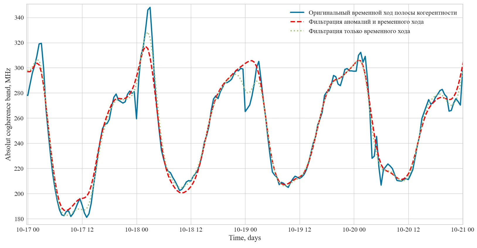
Processing the components of the series, in the authors’ assessment, approximates sharp jumps of the coherence bandwidth more accurately. As the number of shifts approaches 150, both R² and the RMS deviation decrease, so the number of shifts is limited to 150. The best results for all samples lie between 50 and 80 shifts. The best result — R² 90 % and an RMS deviation of 11.1 MHz — came from the 70-day sample with shifts with subtraction, the worst from the 50-day sample. Shift features raised forecast accuracy by about 11 % and lowered the RMS deviation by 8 MHz; processing the trend and variations raised R² by 4 % and lowered the RMS deviation by 2 MHz.
Authors’ conclusions
The task of intelligent processing of diurnal variations of the coherence bandwidth for forecasting has been solved. Decomposing the series into trend, seasonality and variations with a Hodrick — Prescott filter and an isolation forest, together with shift-with-subtraction features, improves the accuracy of an XGBoost forecast. The work was supported by Russian Science Foundation grant No 22-19-00073.
Limitations
The coherence bandwidth is proportional to f^(3/2), but the frequency for which the series was computed is not given, nor are the source of the TEC — a station or the GNSS network — the sampling step and the forecast horizon; the split into training and test parts is not described either. So 50–80 shifts cannot be converted into hours, and an RMS deviation of 11.1 MHz cannot be compared with other work.
The role of the Hodrick — Prescott filter is described inconsistently: in the methods as smoothing long-term cyclic components, in the conclusion as approximating short-term variations due to ionospheric inhomogeneities. The isolation forest is called a random-forest algorithm, although it is a separate ensemble of isolation trees. “An 11 % increase in accuracy” is not specified — percentage points of R² or a relative figure.
Fig. 1 shows that filtering anomalies replaces dips in the original series with a smooth curve — in the first hours of 19 October the original series falls to 265 MHz while the filtered one rises to 305 MHz — but it is not discussed whether this is an artefact or a real ionospheric feature. Nor is it said whether the RMS deviation was computed against the original or the filtered series: in the latter case part of the gain from processing the components is built into the target itself. Fig. 2 puts 16 series, with R² in per cent and RMS deviation in megahertz, on a single axis, which makes it hard to read.
Novelty
The paper claims the application to the coherence-bandwidth series of a decomposition with a Hodrick — Prescott filter and an isolation forest, and of an XGBoost model on shifts with subtraction.
Heuristics
- [explicit] If outliers are sought in a series with strong daily periodicity — subtract the trend and seasonality first and look for anomalies in the residual, which has no constant components.
- [explicit] If a forecasting model knows nothing of the series’ dynamics — add shift-with-subtraction features (differences), not only the shifts themselves.
- [explicit] If the number of shifts grows — tune it by the metrics on each sample: here the best results for all samples lie between 50 and 80 shifts.
- [reconstructed] If the forecast quantity is computed from another one (here the coherence bandwidth from TEC) — state the conversion parameters, otherwise the result cannot be reproduced or compared.
- [reconstructed] If outlier treatment improves a metric — check the metric against the original series too, otherwise the improvement may be built into the target itself.
In one sentence: Decomposing the diurnal course of the coherence bandwidth into trend, seasonality and residual with an isolation forest, plus shift-with-subtraction features, gives XGBoost a forecast with R² up to 90 % and an RMS deviation of 11.1 MHz, while the conversion frequency, the sampling step and the forecast horizon remain unstated.