Machine learning for forecasting MUF time series of HF radio channels

Problem and relevance

The frequency limits of an HF channel change with the state of the ionosphere, and the optimum working frequency is chosen about 15 % below the maximum usable frequency (MUF). To plan the operation of a radio system in advance, the MUF has to be forecast hours and days ahead rather than minutes. The paper looks at how much such a forecast depends on the preprocessing of the raw MUF series.

Aim and hypothesis

The aim is an algorithm for long-term (from several hours to several days) forecasting of the MUF with machine-learning methods. The tasks are to choose the window and order of the smoothing filter, the way the series is split into training and test samples, and the treatment of outliers. No hypothesis is stated explicitly; in substance the paper tests that smoothing and outlier removal improve the forecast and that XGBoost is more accurate than linear regression.

Materials and methods

The source data are MUF values obtained with a chirp ionosonde diagnosing HF radio channels. The series is smoothed with a Savitzky — Golay polynomial filter. The window length is chosen from the autocorrelation function of the diurnal course as the 95 % confidence interval of the ACF samples, and the filter order from the condition of 95 % cross-correlation between the series before and after filtering. Windows of 15, 17, 19 and 21 samples were compared at orders 1 to 5; each combination is averaged over five splits.

The splits are made with sklearn’s TimeSeriesSplit, so the training part always precedes the test part. Outliers are found with sklearn’s isolation forest: the algorithm gives each sample an “anomaly” score, the researcher picks the threshold according to the level of outliers in the series, and the samples found are then smoothed. Two models are compared: linear regression, as simple and cheap, and XGBoost, as more accurate and more demanding. The quality criteria are the coefficient of determination and the RMS deviation of the forecast from the experimental MUF values.

Results

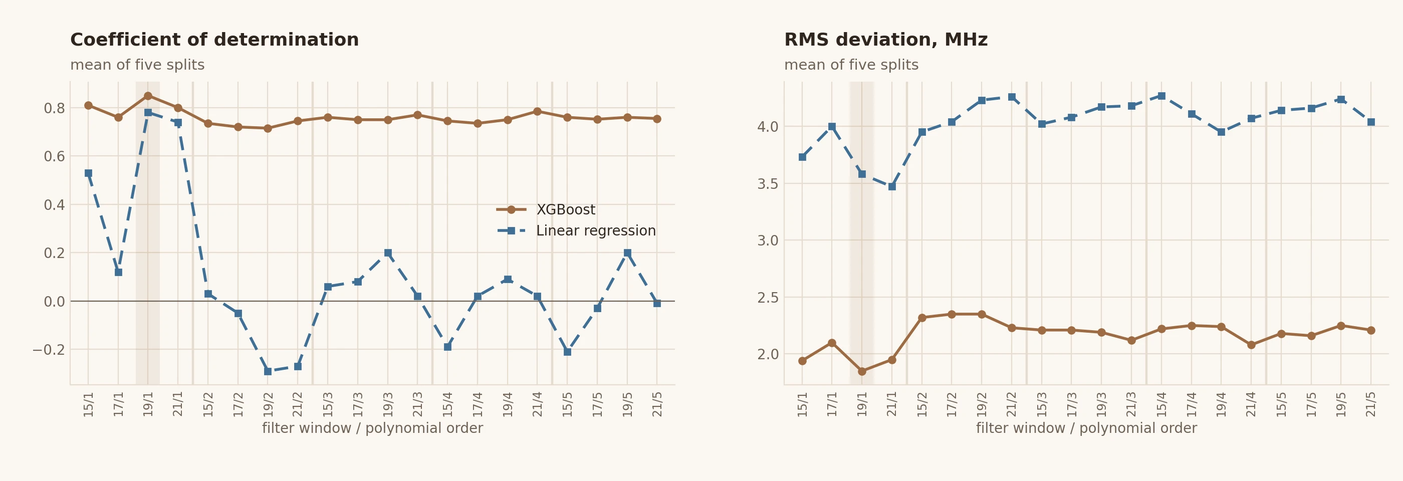
Two plots over twenty filter settings from 15/1 to 21/5. Left, the coefficient of determination: 0.71–0.85 for XGBoost, from −0.29 to 0.78 for linear regression with its maximum at 19/1. Right, the RMS deviation: 1.85–2.35 MHz for XGBoost, 3.5–4.3 MHz for linear regression — Forecast quality at different Savitzky — Golay filter settings. Redrawn from Figs 1 and 2 of the paper; values read off the plots approximately. The 19/1 setting is highlighted.

The coefficient of determination of XGBoost hardly depends on the filter setting and stays at about 0.7–0.85, while that of linear regression ranges from negative values to 0.78 — at most settings the linear model forecasts worse than the plain mean of the series. The best setting is a window of 19 at first order: XGBoost reaches R² 0.86 and an RMS deviation of 1.8 MHz; linear regression also shows its maximum R² at this point but trails XGBoost by about 1.5 MHz in RMS deviation.

On a 12-day stretch the isolation forest marked as outliers single samples within days and a group of samples at the end of the series. Treating the outliers improved the models by 1.5 MHz in RMS deviation and by 0.2 in the coefficient of determination on average. In an example forecast about 1.3 days long, XGBoost had an RMS deviation of 1.8 MHz at R² 0.83, linear regression 3.2 MHz at R² 0.37.

Authors’ conclusions

The optimal ratio of window to filter order is 19/1 by two criteria: the maximum coefficient of determination (0.86) and the minimum RMS deviation (1.8 MHz) for XGBoost. Treating outliers with an isolation forest improves accuracy by 1.5 MHz in RMS deviation and 0.2 in R² on average. For further research into long-term MUF forecasting, XGBoost is the most promising model.

Limitations

The path, the observation period, the sampling step and the sample size are not given; Fig. 3 only suggests that 12 days hold about 3,500 samples, i.e. a step of about 5 minutes. The features the models are trained on are not described, nor is the forecast horizon used when choosing the filter — the example in Fig. 4 covers about 1.3 days. The statement that linear regression also has its minimum RMS deviation at 19/1 is not borne out by Fig. 2: its deviation is lower at 21/1. The isolation-forest threshold is chosen by hand, and the group of “outliers” at the end of the 12-day series may be an edge effect of the smoothing rather than an ionospheric anomaly; this is not discussed. There is no comparison with a simple baseline, such as repeating the previous day’s course.

Novelty

The paper does not claim novelty explicitly. In substance it proposes a preprocessing chain for the MUF series — a Savitzky — Golay filter with an ACF-based window and an isolation forest for outliers — and tests how it affects forecasting with linear regression and XGBoost.

Heuristics

[explicit] If the window of a smoothing filter must not be chosen blindly — take it from the series’ autocorrelation function (the 95 % interval), and the order from how well the correlation between the series before and after filtering is preserved.
[explicit] If a time series is split into training and test samples — split it so that training always precedes testing (TimeSeriesSplit) instead of shuffling samples.
[reconstructed] If a model’s coefficient of determination turns negative — the model forecasts worse than the mean, and tuning it by that metric is pointless; change the model or the features first.
[reconstructed] If outliers cluster at the edge of a series — check for an edge effect of the smoothing before treating them as anomalies of the medium.
[reconstructed] If forecasting models for a diurnal course are compared — add a “same as yesterday” baseline, because a high R² may be explained by the daily periodicity alone.

In one sentence: Smoothing the MUF series with a Savitzky — Golay filter with a window of 19 and removing outliers with an isolation forest give XGBoost a forecast about a day ahead with R² 0.86 and an RMS deviation of 1.8 MHz, while linear regression does no better than the mean at most settings.