Method and algorithm for determining the periods of operational forecasting of HF maximum usable frequency dynamics based on the XGBoost machine-learning algorithm

Problem and relevance

The most reliable HF communication is given by working frequencies of 0.8–0.9 of the maximum usable frequency (MUF), and because of the variability of the ionosphere the MUF is a random dynamic quantity. It is determined by active sensors — vertical ones, covering an area of up to 500 km in radius, and oblique ones, characterising the midpoint of a path. To assign frequencies in advance the MUF has to be forecast, and a forecast with XGBoost raises the question of how far ahead it stays accurate enough.

Aim and hypothesis

The aim is an algorithm for estimating the optimal periods of forecasting the MUF of ionospheric HF links based on XGBoost, and its experimental verification on a 2,600 km mid-latitude path. No hypothesis is stated explicitly; in substance the paper tests that tuning the hyperparameters lengthens the period during which the forecast error stays below a threshold.

Materials and methods

The MUF is computed from an oblique-sounding ionogram cleaned of interference: consecutive partial channels are counted from right to left on the frequency grid, and the frequency of the last sample is taken as the MUF. The values are accumulated in a database. The series covers 30 days at a 5-minute step, 8,640 values in all; in preprocessing, gaps are interpolated and anomalous values evened out. The loss metric is the mean absolute error (MAE), as the easiest to interpret and less sensitive to large deviations; quality is also judged by RMSE and the coefficient of determination R².

The paper derives the objective function of gradient boosting with regularisation and a second-order expansion of the loss, and lists the XGBoost hyperparameters. They are tuned with the hyperopt library — random search, TPE and adaptive TPE: n_estimators, eta, gamma, max_depth, lambda, alpha, colsample_bytree, colsample_bylevel, min_child_weight and subsample. Trained models are checked by MAE and R² and saved to a database as .sav files; when forecasting, the algorithm goes through the models and picks the one within the metric thresholds, then checks stability with repeated runs.

The samples are split by days: the test part grows from one day until the MAE exceeds a threshold of 1 MHz — set by the power of the random component of the MUF series found in earlier studies — and the training part shrinks accordingly from 29 days. Models with and without hyperparameter tuning are compared.

Results

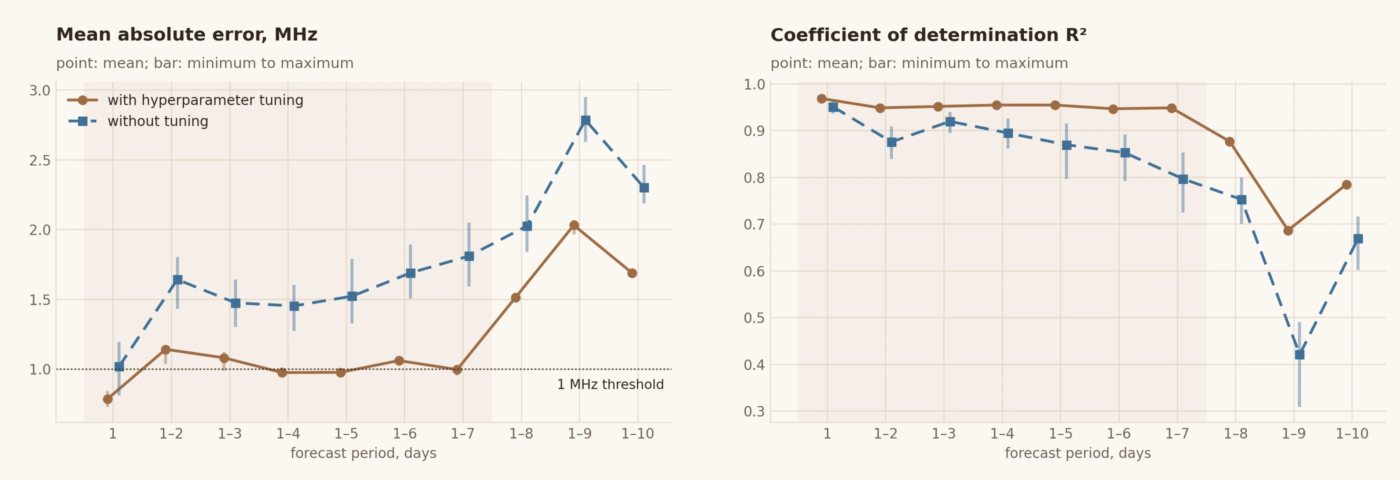
Two plots over ten forecast periods. Left, MAE: with tuning from 0.79 MHz for 1 day to about 1.0 MHz for 1–7 days and 1.5–2.0 MHz for 8–10 days; without tuning from 1.0 to 1.8 MHz and up to 2.8 MHz. Right, R²: with tuning 0.95–0.97 up to seven days, without tuning from 0.95 down to 0.80 — Forecast metrics for periods from 1 to 1–10 days. Redrawn from Fig. 2 of the paper: the values were recovered from the PDF's vector graphics. The 1–7 day range the paper calls optimal is shaded.

At eight days and beyond, the metrics jump sharply past the thresholds. The longest period with tuning is seven days: mean MAE 0.99 MHz, R² 0.95. Without tuning the longest period is one day: MAE about 1 MHz, R² 0.95. The best period is one day: minimum MAE 0.72 MHz, mean 0.78 MHz, at most 0.84 MHz, R² 0.97. In a one-day forecast, tuning gains 0.25 MHz in MAE and 2 % in R².

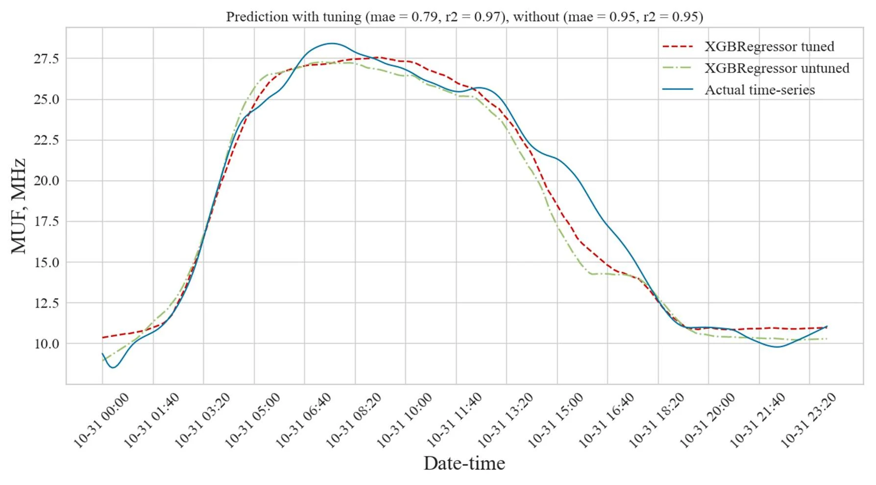
The diurnal course of the MUF on 31 October from 9 to 28 MHz: the actual series and two forecasts; the plot title gives MAE 0.79 and R² 0.97 with tuning, MAE 0.95 and R² 0.95 without. The forecasts depart most from the actual series between 13:00 and 17:00, as the MUF falls — A one-day MUF forecast by the model with and without hyperparameter tuning, and the actual course with its random component smoothed — Fig. 3 of the paper.

The error plot shows the largest forecast scatter at MUF values of 14–18 MHz between 11:00 and 17:00 — from the afternoon to sunset, which agrees with the author’s earlier studies and those of others.

Author’s conclusions

An algorithm for estimating the optimal periods of MUF forecasting with XGBoost has been developed. Models with tuned hyperparameters are 25 % better in MAE (mean 1.43 MHz) and 8 % better in R² (mean 0.94) over periods of one to seven days. The shortest forecast period is one day (MAE 0.78 MHz, R² 0.97), the longest seven days (MAE 0.99 MHz, R² 0.95); compared with the untuned model the forecast period is increased sevenfold. A class of Python programs has been created for practical use.

Limitations

The paper’s main numbers are borne out by Fig. 2: values recovered from the vector graphics give, for one day, an MAE of 0.79 MHz with a minimum of 0.73 and a maximum of 0.84, and for 1–7 days 1.00 MHz at R² 0.95. The summary averages do not agree: by Fig. 2 the mean MAE over the 1–7 day periods is about 1.0 MHz with tuning and about 1.5 MHz without — a gain of about a third, not 25 % — and where the mean of 1.43 MHz comes from is unclear. The 1–2 day period is excluded from the optimal ones for exceeding 1 MHz (mean 1.14), although the 1–3 and 1–6 day periods also have means above the threshold — 1.08 and 1.06 MHz.

The model is selected by MAE and R² and assessed by the same metrics; a separate validation part that takes no part in the selection is not described, so the estimates are probably optimistic. The model’s features are not described — it is only said that the independent variable is time; a decision tree does not extrapolate beyond its training values, and when forecasting days ahead the model apparently reproduces a typical diurnal course. There is no comparison with such a simple baseline — the mean diurnal course or the previous day’s course — and a high R² with the MUF ranging from 10 to 28 MHz is largely explained by the daily periodicity itself. The actual course in Fig. 3 has its random component smoothed, i.e. the metrics are not computed on the raw series.

The path and the observation dates are not named; 30 days are a single season, and the seven-day conclusion applies to it. The text has inaccuracies: the number of tree leaves is called the “number of petals”, L1 and L2 regularisation are listed in reverse order relative to alpha and lambda, equation number (5) is repeated and (6) is missing.

Novelty

The paper claims a method and algorithm for determining optimal periods of MUF forecasting with XGBoost and automatic hyperparameter tuning, and an experimentally established sevenfold increase of the forecast period.

Heuristics

[explicit] If there are many hyperparameters — tune them automatically (hyperopt, TPE) rather than by hand.
[explicit] If the limiting forecast horizon is sought — extend the test part day by day until the error exceeds a threshold justified by the power of the series’ random component.
[explicit] If a model’s result varies from run to run — check stability with repeated runs and look at the spread of the metrics, not at a single value.
[reconstructed] If a model is selected by its metrics — keep a separate part of the data that takes no part in the selection, otherwise the final estimate will be inflated.
[reconstructed] If a tree ensemble forecasts a continuous quantity — expect a stepped forecast: on the error plot it shows as horizontal shelves where the forecast stays constant while the MUF changes.

In one sentence: XGBoost with tuned hyperparameters keeps the mean absolute error of an MUF forecast near 1 MHz for up to seven days against one day without tuning, but selecting the model by the same metrics, the lack of a baseline and a smoothed target make these numbers an upper estimate.