ionozond: A Chirp Ionosonde Console Recovered from Its Binary
The source of an oblique chirp-sounding console was lost; only the built binary remained. How the program was recovered from it and shown to match the original, which quirks had to be kept, why a 37 KB file sits beside each 80 MB capture, and what the console does now — from an ionogram drawn during reception to a check of the station schedule.
Oblique chirp sounding measures the ionosphere along a path between a transmitter and a receiver. The transmitter sweeps the HF band with a linearly changing frequency; the receiver multiplies what it hears by the same reference sweep and records the beat signal. The recording yields an ionogram — signal strength against frequency and echo delay — and the ionogram shows which band of frequencies the path carries. The main path here is Cyprus — Yoshkar-Ola.
transmitter  ──▶  receiver  ──▶  .lfs capture  ──▶  .lfp products  ──▶  console
                 (acquisition)      80 MB             ~40 kB
The operator’s console is a Qt5 and Qwt program that shows ionograms, keeps the station schedule and starts reception. Its source was lost: only the built program dsChirp remained. ionozond began on 25 August with recovering it, and in a month and a half grew into a suite of acquisition, console, formats, tools and documentation — 105 commits.
Recovery from the binary
What made recovery possible was that the binary had not been stripped: class names, method signatures and Qt’s meta-object data survived. The program was also not built as position-independent, so its function addresses are known in advance.
That turned the original into a reference. It runs in the same container as the reconstruction, and its functions are called inside it under gdb. There is no debug information, so each call has to be cast by hand: set $f = (double (*)(double*, int*))getMedian. A separate script runs the original’s whole interface headless with the test settings.
Verification worked at three levels. The spectrum calculation was rewritten and checked against an independent NumPy implementation on a real capture — they agree to 1.7·10⁻¹³ relative, which is only the summation order of the FFT. The configuration file the program generates matches the original’s byte for byte. Ionogram rendering was compared on real captures.
Quirks kept on purpose
An exact copy must also repeat what a natural reimplementation would do differently. Each such place is recorded in docs/reverse-engineering.md and pinned by a test.
- A median that is not a median for an odd count.
getMedianalways takes half the sum of the lower half’s maximum and the element atn/2. Called under gdb for{5, 1, 9, 3, 7, 2, 8}, the original returned 4, where the median is 5. Spectrum lengths are powers of two, so this never shows in practice, but it is reproduced exactly. - A periodic Hann window: divided by n, not n − 1, as in
scipy.signal.get_window('hann', n, fftbins=True)rather thannumpy.hanning(). The window’s step is narrowed tofloatas in the original, so the window matches bit for bit.
One of the original’s bugs was fixed rather than reproduced. The parameters dialog wrote the key colormap_gradient, while the main window read colormap_gradinet, with a typo. The colour-scale choice was saved but had no effect on the plots. The fix is marked DSCHIRP_FIX_GRADIENT_TYPO in the code, with the original behaviour described in a comment.
Another inherited inaccuracy surfaced later: the original’s path-length formula lacks cos(Δλ) in its second term. For Cyprus that gives 2542 km instead of 2591 along the great circle, for Magadan 4414 km instead of 5476. Because of it, the delay-axis labels on the power-delay panel disagreed with the data by several milliseconds. The console now computes the correct great circle; the original’s formula is kept as a separate function, and a test shows it still reproduces the original’s window.
Two formats
.lfs is the raw capture: a 512-byte header and a stream of complex float32 I/Q samples. One 250-second sounding takes 80 MB, and at a 300-second repetition period one station produces about 23 GB a day. The header layout was checked field by field against two real captures — 31 offset assertions. Files of the newer version 1.1 are refused, as the original refused them, and this is reproduced on purpose.
.lfp is the products file beside a capture: the ionogram, the signal and noise spectrum, the power-delay profile and the band edges. The console reads it first, so the heavy processing happens once:
cyprus1_20191023_071510.lfs    76.3 MB
cyprus1_20191023_071510.lfp    37.0 kB      2112x smaller
An HDF5 archive compatible with chirpsounder2 is written beside each capture too; it is now the main one, and the raw capture is optional. Raw captures have a retention period and are removed only after their products have been verified. Synchronisation with network storage also removes files only after the copy has been checked.
Acquisition
The signal path from the radio to the file was rewritten in Python 3. Most of the late-August commits are about real hardware being harder than expected. The radio’s clock is set even without GPS, and the receiver checks which clock to trust rather than assuming GPS is right. Lost samples turned out to come from the network card’s receive ring overflowing — its size is now raised and kept across reboots. Samples lost to an overflow are filled with zeros so that the time base does not slip, and a capture with overflows counts as degraded, not failed. The receiver runs as a systemd service.
The console today
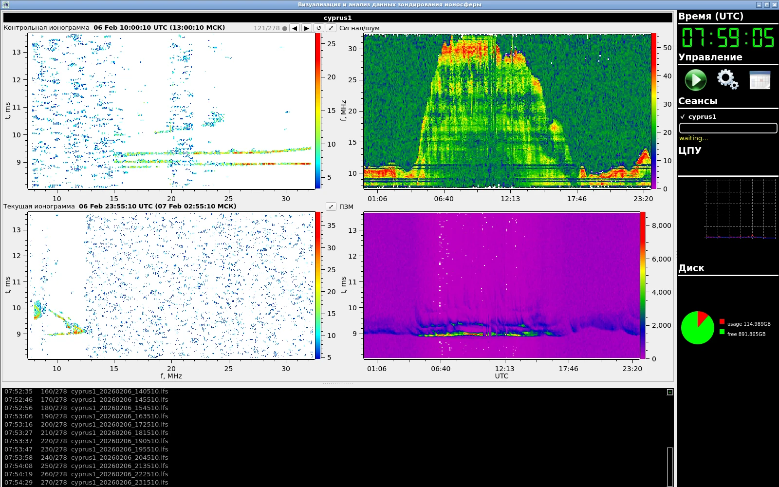
The console shows each station as two ionograms — the control one and the current one — and two panels over the day. Capture times are given in UTC and Moscow time: captures are named and scheduled in UTC, while people at the station keep Moscow time.
As in the original, the current ionogram is now drawn during reception, left to right. Every two seconds the console finds the growing capture and computes only the new columns, with the same arithmetic as the products builder. On a 2019 capture the result matches the builder to 6·10⁻⁶ dB, so when the finished .lfp replaces the live picture at the end of a sounding, nothing jumps. A test feeds a capture in uneven pieces and requires the result to equal the one-pass picture bit for bit.
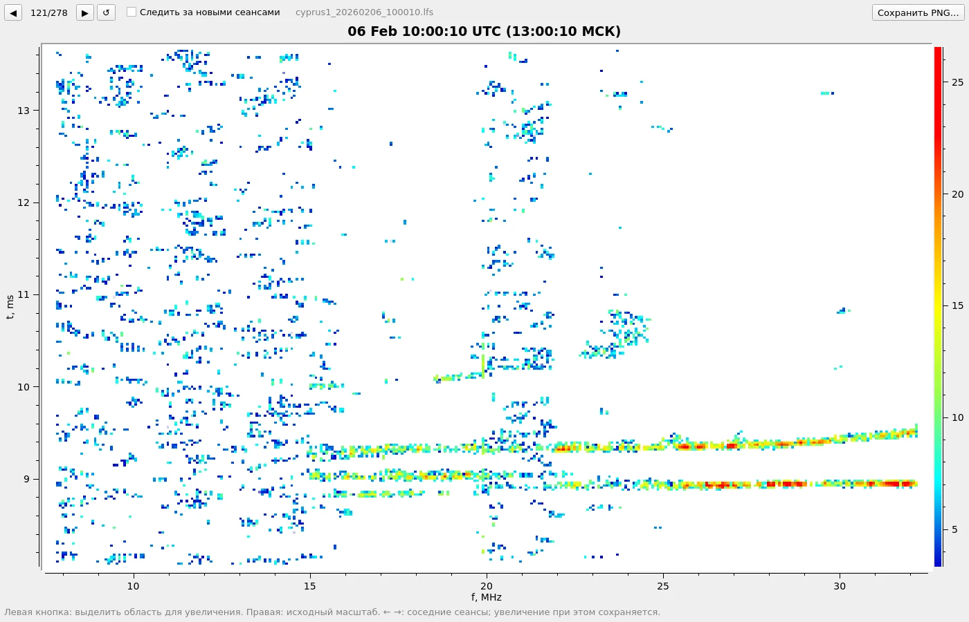
The FFT length is set per station. An ionogram cell is k·N/f_IF in frequency by f_IF/(k·N) in delay, so one length cannot suit stations with different sweep rates. 16,384 points give a 41 kHz × 7.3 km cell at 100 kHz/s but 205 kHz × 1.5 km at 500 kHz/s: an echo that moves by 5 µs leaves its cell. At 4,096 points the cell is 51 kHz × 5.9 km — close to the original’s shape.
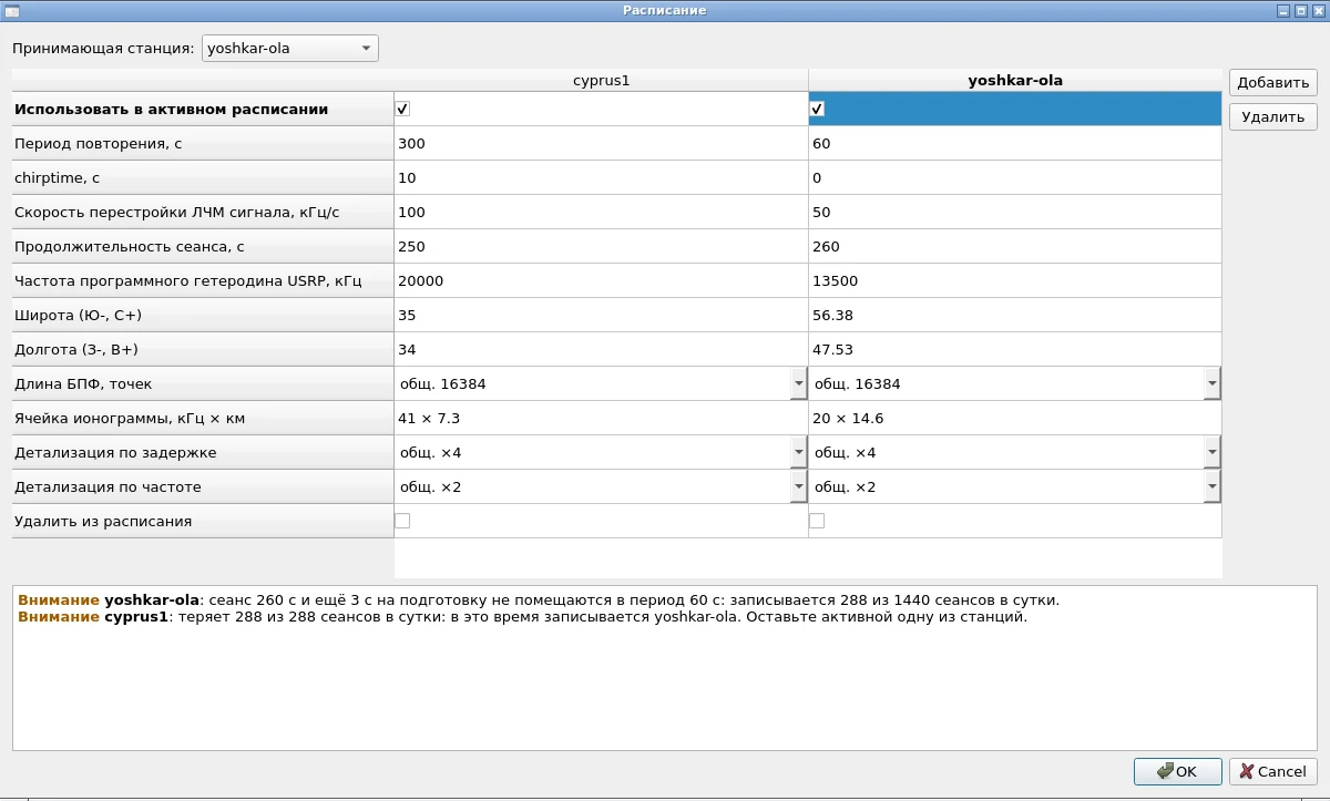
One radio follows one sweep, so a station whose sounding fell during another’s recording was simply not recorded — and nothing said so. Now the check replays a day by the same selection rules as the receiver itself, names the lost soundings and the station holding the radio, and offers a fix verified by re-simulation. It also catches what the configuration file cannot take: decimal commas, leading zeros, quotes in names, a non-positive period.
A document on the physics of chirp ionograms
Beside the code sits a document, “Oblique Chirp Ionograms”: how an ionogram forms, what its traces mean and where the console can mislead. The document has 16 parts; the new one, Part 11, is about group-delay dispersion (GDD): the slope of a trace, dτ/df, which decides how wide a band the path carries undistorted.
The numbers come from this path: 19,033 one-megahertz slope estimates of the lower 1F ray, from 583 soundings on 4–9 February 2026, with the MUF between 18 and 32.4 MHz. The median follows 7.5·(1/√(1 − f/MUF) − 1) µs/MHz. On the console’s screen this dispersion is invisible: even 35 µs/MHz lifts a trace by only 1.4 µs across a 41 kHz column — about 6 % of a cell. The document’s interactive models have moved into a separate playground, the subject of the next breakdown.
The document is maintained like code. The latest commit fixes places that its own tables and formulas contradict: for example, doubling the FFT length doubles the frequency step rather than halving it. Another note explains why two ISZF transmitters, in Magadan and Norilsk, are not heard in Yoshkar-Ola: their antennas point at Irkutsk.
Running it in a browser
Docker is all it takes. The console runs on a virtual display inside a container and is driven from an ordinary browser over noVNC. The capture directory is mounted read-only, so the program cannot change the archive. The screenshots in this breakdown were taken exactly that way, on the captures of 6 February.
Conclusions
- A binary that has not been stripped is almost source code: class names and function addresses turn the original into a reference that can be called piece by piece.
- A copy’s fidelity is shown not by pictures looking alike but by comparison: byte for byte for the configuration, numerically for the spectra, and a test for each quirk.
- The original’s quirks are worth repeating and documenting; fixes should be explicit and marked in the code.
- A products file 2000 times smaller than the capture moves the heavy processing to where it is done once.
- A schedule check turns a silent loss of soundings into a warning with a ready fix.
Availability
The source code is open. The third-party sources the capture format was checked against are not in the repository: they are under someone else’s licence. The original binary is not in the repository either.
- Source code: github.com/nikita-konkin/ionozond
- Interactive models: konkin-nikita.ru/ionozond-playground